So guys in today’s blog we will see how we can perform Google’s stock price prediction using our Keras’ LSTMs model trained on past stocks data. So without any further due, Let’s do it…
Step 1 – Importing required libraries.
import numpy as np
import pandas as pd
import matplotlib.pyplot as plt
from sklearn.preprocessing import MinMaxScaler
from tensorflow.keras.models import Sequential
from tensorflow.keras.layers import LSTM,Dropout,Dense
Step 2 – Reading our training data.
dataset_train = pd.read_csv('Google_Stock_Price_Train.csv')
training_set = dataset_train.iloc[:, 1:2].values

sc = MinMaxScaler(feature_range = (0, 1))
training_set_scaled = sc.fit_transform(training_set)

X_train = []
y_train = []

for i in range(60, 1258):
    X_train.append(training_set_scaled[i-60:i, 0])
    y_train.append(training_set_scaled[i, 0])
- Here we are reading the input train data.
- We are just taking the first column here which is the ‘open’ column.
- Then we are initializing the MinMaxScaler to scale our data between 0 and 1.
- After that, we initialized two arrays X_train and y_train.
- The first entry in the X_train would be an array of the first 60 open stock prices and the first entry in the y_train will be the 61st value of open stock price. It means that we want our model to predict the 61st value of stock price when we provide it with the previous 60 values.
- In this way, we keep on building our X_train and y_train.
Step 3 – Getting our training data in shape.
X_train, y_train = np.array(X_train), np.array(y_train)
X_train = np.reshape(X_train, (X_train.shape[0], X_train.shape[1], 1))
- Here we are converting our lists to arrays.
- In the 2nd step, we are adding a dummy dimension in the end because Keras models require the data in this format only.
Step 4 – Creating the Stock Price Prediction model.
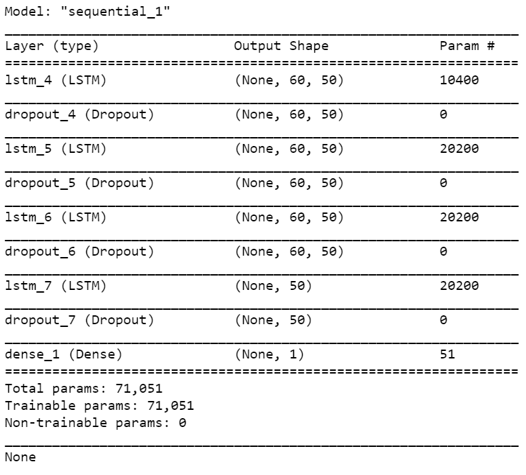
regressor = Sequential()

regressor.add(LSTM(units = 50, return_sequences = True, input_shape = (X_train.shape[1], 1)))
regressor.add(Dropout(0.2))

regressor.add(LSTM(units = 50, return_sequences = True))
regressor.add(Dropout(0.2))

regressor.add(LSTM(units = 50, return_sequences = True))
regressor.add(Dropout(0.2))

regressor.add(LSTM(units = 50))
regressor.add(Dropout(0.2))

regressor.add(Dense(units = 1))

regressor.compile(optimizer = 'adam', loss = 'mean_squared_error')

print(regressor.summary())
- Our Sequential model consists of 4 LSTM layers with 50 units each.
- After these LSTM layers, we have a Dense layer.
- We are using Adam optimizer here and the loss we are using is Mean Squared Error.
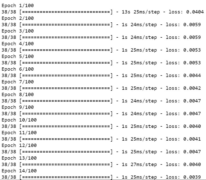
Step 5 – Training the Stock Price Prediction model.
regressor.fit(X_train, y_train, epochs = 100, batch_size = 32)
- Training our model for 100 epochs.
- The batch size which we have taken is 32.
- You can also experiment with these values.
Step 6 – Reading the test data.
dataset_test = pd.read_csv('Google_Stock_Price_Test.csv')
real_stock_price = dataset_test.iloc[:, 1:2].values
- Now let’s read the test data to perform our predictions.
Step 7 -Getting the Stock Price Predictions on test data.
dataset_total = pd.concat((dataset_train['Open'], dataset_test['Open']), axis = 0)
inputs = dataset_total[len(dataset_total) - len(dataset_test) - 60:].values

inputs = inputs.reshape(-1,1)
inputs = sc.transform(inputs)

X_test = []

for i in range(60, 80):
    X_test.append(inputs[i-60:i, 0])

X_test = np.array(X_test)
X_test = np.reshape(X_test, (X_test.shape[0], X_test.shape[1], 1))

predicted_stock_price = regressor.predict(X_test)
predicted_stock_price = sc.inverse_transform(predicted_stock_price)
- Concatenating the test ‘Open’ column with the train ‘Open’ column row-wise.
- The step we did above was just to take the last 60 values from the train data and also add that to the test data.
- Then we are reshaping it to have just one column and as many rows.
- Scaling it using MinMaxScaler.
- Then we are creating the test data as we did for the train data.
- And finally, we are making predictions.
NOTE – What we are doing above is we are first taking the last 60 open values from the train and making predictions from it for the 61st value. Then what we will do is we will drop the 0th open value and now our input array will be 1st open value to the 61st open value (60 values) and we will predict the 62nd open value and like this, we will keep on predicting the next value and take that for predicting next values.
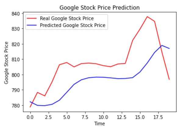
Step 8 – Plotting the predictions and real data.
plt.plot(real_stock_price, color = 'red', label = 'Real Google Stock Price')
plt.plot(predicted_stock_price, color = 'blue', label = 'Predicted Google Stock Price')
plt.title('Google Stock Price Prediction')
plt.xlabel('Time')
plt.ylabel('Google Stock Price')
plt.legend()
plt.show()
- Here we are simply plotting our predictions in the blue curve.
- The red curve represents its true value, which means what it should be exactly.
- We can see that our model is not that perfect but still it is capable of catching the spikes (where the curve starts to go up).
Download the Source Code…
Do let me know if there’s any query regarding Stock Price Prediction by contacting me on email or LinkedIn.
So this is all for this blog folks, thanks for reading it and I hope you are taking something with you after reading this and till the next time 🙂
NOTE – And yes one more thing please do not invest your money in the stock market on basis of just these models or predictions. These are just for educational purposes. ??
Read my previous post: IMAGE CAPTIONING
Check out my other machine learning projects, deep learning projects, computer vision projects, NLP projects, Flask projects at machinelearningprojects.net.