
So in today’s blog, we are going to perform the weight category prediction of a person given height, weight, and gender with the help of the Random Forest algorithm.
This is going to be a very interesting blog, so without any further due, let’s do it…
Checkout the video here – https://youtu.be/YmZe9lreH4M
Code for weight category prediction…
import numpy as np
import pandas as pd
import seaborn as sns
import matplotlib.pyplot as plt
from sklearn.preprocessing import StandardScaler
from sklearn.ensemble import RandomForestClassifier
from sklearn.model_selection import GridSearchCV, train_test_split
from sklearn.metrics import classification_report,confusion_matrix,accuracy_score
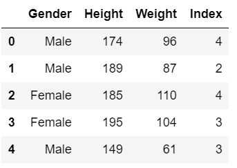
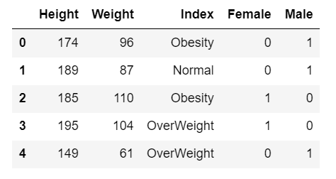
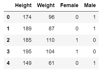
data = pd.read_csv('500_Person_Gender_Height_Weight_Index.csv')
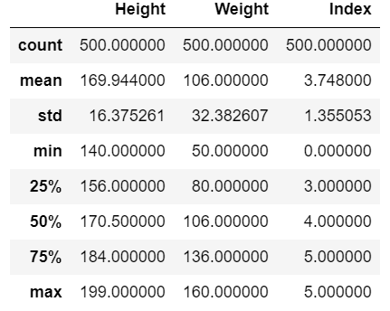
print(data.describe())
def give_names_to_indices(ind):
if ind==0:
return 'Extremely Weak'
elif ind==1:
return 'Weak'
elif ind==2:
return 'Normal'
elif ind==3:
return 'OverWeight'
elif ind==4:
return 'Obesity'
elif ind==5:
return 'Extremely Obese'
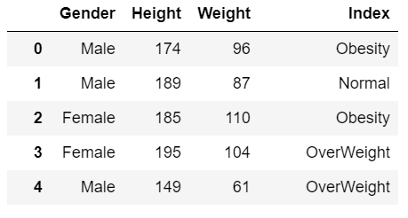
data['Index'] = data['Index'].apply(give_names_to_indices)
sns.lmplot('Height','Weight',data,hue='Index',size=7,aspect=1,fit_reg=False)
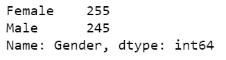
people = data['Gender'].value_counts()
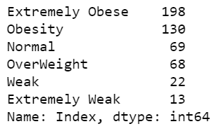
categories = data['Index'].value_counts()
# STATS FOR MEN
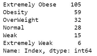
data[data['Gender']=='Male']['Index'].value_counts()
# STATS FOR WOMEN
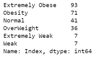
data[data['Gender']=='Female']['Index'].value_counts()
data2 = pd.get_dummies(data['Gender'])
data.drop('Gender',axis=1,inplace=True)
data = pd.concat([data,data2],axis=1)
y=data['Index']
data =data.drop(['Index'],axis=1)
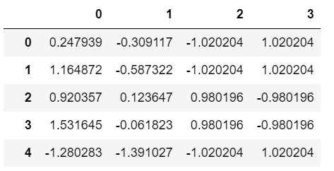
scaler = StandardScaler()
data = scaler.fit_transform(data)
data=pd.DataFrame(data)
X_train, X_test, y_train, y_test = train_test_split(data, y, test_size=0.3, random_state=101)
param_grid = {'n_estimators':[100,200,300,400,500,600,700,800,1000]}
grid_cv = GridSearchCV(RandomForestClassifier(random_state=101),param_grid,verbose=3)
grid_cv.fit(X_train,y_train)
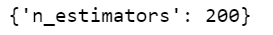
print(grid_cv.best_params_)
# weight category prediction
pred = grid_cv.predict(X_test)
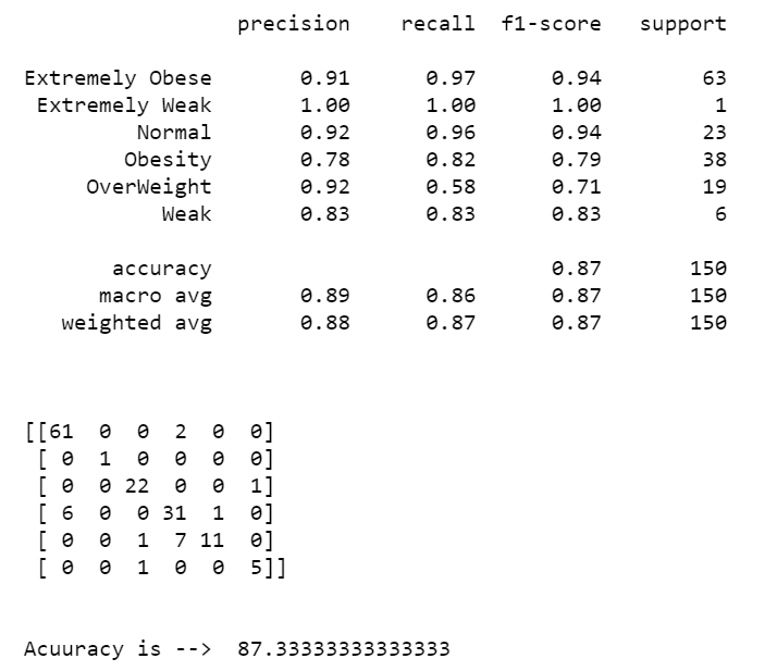
print(classification_report(y_test,pred))
print('\n')
print(confusion_matrix(y_test,pred))
print('\n')
print('Acuuracy is --> ',accuracy_score(y_test,pred)*100)
print('\n')
def lp(details):
gender = details[0]
height = details[1]
weight = details[2]
if gender=='Male':
details=np.array([[np.float(height),np.float(weight),0.0,1.0]])
elif gender=='Female':
details=np.array([[np.float(height),np.float(weight),1.0,0.0]])
y_pred = grid_cv.predict(scaler.transform(details))
return (y_pred[0])
#Live predictor
your_details = ['Male',175,80]
print(lp(your_details))
- Line 1-8 – Importing required libraries.
- Line 10 – Reading our data.
- Line 11 – Describing our data.
- Line 13-25 – Create a function to convert numerical values of the Index column to categorical values.
- Line 28 – Apply this function to make changes.
- Line 30 – Let’s plot height vs weight and color them according to their weight category. We are using sns.lmplot which is just a scatter plot or we can say a regression plot.

- Line 32 – Let’s analyze the value counts of the Gender column.
- Line 34 – Let’s analyze the value counts of the Index column.
- Line 36-40 – Let’s analyze weight category distribution according to gender.
- Line 42-44 – Now when we are done with data exploration, let’s start building the model. We can’t give our model categorical features. so we will create dummy variables out of the Gender column, then we will drop the original gender column and merge these 2 dummy variables with our main dataframe.

- Line 46 – Creating y data which will be our Index column, because this is what we want our model to predict. (Output values)
- Line 47 – Creating X data on which our model will be trained. (Input values)
- Line 49-51 – We are declaring a Standard Scaler and scaling our data to bring everything on the same scale /range. This will help increase our model’s accuracy and will also help in faster training.
- Line 53 – Let’s split our data for training and testing purposes in 70% and 30% proportions respectively.
- Line 55-56 – We could have simply declared our Random forest model with any no. of estimators but by using Grid Search CV we can train our random forest model on multiple n_estimators values like firstly random forest will have n_estimators as 100, the second time it will have it as 200 and so on and we can check that which n_estimator is giving highest accuracy. grid_cv will automatically become the best random forest model.
- Line 58 – Fitting our training data on weight category prediction model.
- Line 60 – Let’s see the best parameters.
- Line 62 – Let’s make weight category predictions on test data.
- Line 65- 70 – Let’s print the classification report, confusion matrix, and accuracy score of our weight category prediction model.
- Line 72-83 – A function that will perform all the preprocessing for live prediction in the next step.
- Line 87-89 – Live prediction. Just make an array ‘your_details’ with the first element as gender, second as height, and third as weight and pass it to the function above for preprocessing and predictions.
Download the Source Code…
Do let me know if there’s any query regarding weight category prediction by contacting me on email or LinkedIn.
So this is all for this blog folks, thanks for reading it and I hope you are taking something with you after reading this and till the next time ?…
Read my previous post: BANKNOTE AUTHENTICATION USING RANDOM FOREST
Check out my other machine learning projects, deep learning projects, computer vision projects, NLP projects, Flask projects at machinelearningprojects.net.
Hi I have live data for Regression problem. eVEN AFTER USING H2o, Pycaret and all possible regression models I m not getting best result.
I used Deep. Then used normalization etc.
Also did feature engg with reduced features.
Can you help please ..
Try Lasso Regression, Ridge Regression, and XGBoost Regressor.
please upload input files also
https://github.com/sharmaji27/Weight-Category-prediction-using-Random-Forest