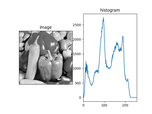
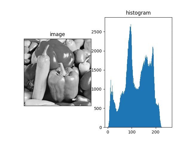
In today’s very short blog we will see that how we can plot a histogram of a grayscale image.
The first way is using NumPy and the second way is using matplotlib. This is going to be a very interesting blog, so without any further due, Let’s do it…
Step 1 – Import the libraries required for the histogram of a grayscale image.
import cv2
import matplotlib.pyplot as plt
import numpy as np
Step 2 – Let’s read the image.
imgpath = "4.2.07.tiff"
img = cv2.imread(imgpath,0)
- Here while reading the image, we passed the second argument as 0 to read the image as a grayscale image.

Step 3 – Let’s plot the image and the histogram of a grayscale image.
Syntax: numpy.histogram(a, bins=10, range=None, normed=None, weights=None, density=None)
Parameters:
| data | Input data. The histogram is computed over the flattened array. |
| bins | int or sequence or str defines the number of equal-width bins in a range, default is 10 |
| range | The lower and upper range of the bins. If not provided, range is simply (a.min(), a.max()). Values outside the range are ignored. |
| normed | optional parameter same as density attribute, gives incorrect result for unequal bin width |
| weights | optional parameter defines array of weights having same dimensions as data |
| density | optional parameter if False result contains number of samples in each bin, if True result contain probability density function at bin |
plt.subplot(1,2,1)
plt.imshow(img,cmap='gray')
plt.title('image')
plt.xticks([])
plt.yticks([])

plt.subplot(1,2,2)
hist,bin = np.histogram(img.ravel(),256,[0,255])
plt.xlim([0,255])
plt.plot(hist)
plt.title('histogram')

plt.show()
- img.ravel is basically used to flatten the 2-D matrix(grayscale image) to a 1-D array.
- Now we will be having our image as something like [125,113,8,45,63…] with no. of elements as n*m where n is the height of the grayscale image and m is the width of the grayscale image.
- Read more about np.histogram here.

Let’s see the whole code of 1st way using NumPy…
import cv2
import matplotlib.pyplot as plt
import numpy as np

imgpath = "test.tiff"
img = cv2.imread(imgpath,0)

plt.subplot(1,2,1)
plt.imshow(img,cmap='gray')
plt.title('image')
plt.xticks([])
plt.yticks([])

plt.subplot(1,2,2)
hist,bin = np.histogram(img.ravel(),256,[0,255])
plt.xlim([0,255])
plt.plot(hist)
plt.title('histogram')
plt.show()
Now let’s see the whole code of 2nd way using matplotlib.
import cv2
import matplotlib.pyplot as plt

imgpath = "test.tiff"
img = cv2.imread(imgpath,0)

plt.subplot(1,2,1)
plt.imshow(img,cmap='gray')
plt.title('image')
plt.xticks([])
plt.yticks([])

plt.subplot(1,2,2)
plt.hist(img.ravel(),256,[0,255])
plt.title('histogram')

plt.show()

Do let me know if there’s any query regarding the histogram of a grayscale image by contacting me on email or LinkedIn.
So this is all for this blog folks, thanks for reading it and I hope you are taking something with you after reading this and till the next time ?…
Read my previous post: HOW TO PERFORM MORPHOLOGICAL OPERATIONS LIKE EROSION, DILATION, AND GRADIENT IN PYTHON USING OPENCV
Check out my other machine learning projects, deep learning projects, computer vision projects, NLP projects, Flask projects at machinelearningprojects.net.


