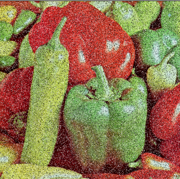
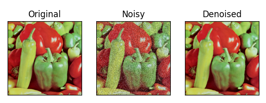
In this blog what we will be seeing will not be something less than magic. You will be amazed after watching the power of Median Blur. So without any further due, let’s do it.
Step 1 – Import all the required packages.
import cv2
import matplotlib.pyplot as plt
import numpy as np
import random
Step 2 – Reading our image.
img = cv2.imread('test.tiff')
img = cv2.cvtColor(img, cv2.COLOR_BGR2RGB)

Step 3 – Creating a black image.
noisy = np.zeros(img.shape, np.uint8)
- Here we have just initialized a black image of same dimensions as of our original image.
- We will be creating our noisy image out of it.
Step 4 – Actually creating the noisy image.
p = 0.2

#traversing throughout the image pixels
for i in range(img.shape[0]): #rows
    for j in range(img.shape[1]): #cols
        r = random.random()
        if r < p / 2:
            noisy[i][j] = [0, 0, 0] #black noise
        elif r < p:
            noisy[i][j] = [255, 255, 255] #white noise
        else:
            noisy[i][j] = img[i][j] #original image pixel
- In the first line, we have just set a random variable p/probability as 0.2.
- Then we will start traversing through the image pixels.
- Then we will take a random value r using random.random() and check if that’s less than p/2 then add a black/pepper noise (0,0,0).
- Else if the random r value is greater than p/2 and less than p then add a white/salt noise.
- Else put the pixel from the original image there.
- 98% of the time it will be the else case (pixel from the original image).

Step 5 – Applying Median Blur to denoise the image.
Syntax: cv2.medianBlur(src, dst, ksize)
Parameters:
| src | A Mat object representing the source (input image) for this operation. |
| dst | A Mat object representing the destination (output image) for this operation. |
| ksize | A Size object representing the size of the kernel. |
# median blur
denoised = cv2.medianBlur(noisy, 5)
Note: Read more about Median Blur in my blog on Blurrings.
Step 6 – Visualizing the results.
output = [img, noisy, denoised]

titles = ['Original', 'Noisy', 'Denoised']

for i in range(3):
    plt.subplot(1, 3, i + 1)
    plt.imshow(output[i])
    plt.title(titles[i])
    plt.xticks([])
    plt.yticks([])
plt.show()

Let’s see the whole code…
import cv2
import matplotlib.pyplot as plt
import numpy as np
import random

img = cv2.imread('test.tiff')
img = cv2.cvtColor(img, cv2.COLOR_BGR2RGB)

noisy = np.zeros(img.shape, np.uint8)

p = 0.2

# traversing throughout the image pixels
for i in range(img.shape[0]):  # rows
    for j in range(img.shape[1]):  # cols
        r = random.random()
        if r < p / 2:
            noisy[i][j] = [0, 0, 0]  # black noise
        elif r < p:
            noisy[i][j] = [255, 255, 255]  # white noise
        else:
            noisy[i][j] = img[i][j]  # original image pixel

# median blur
denoised = cv2.medianBlur(noisy, 5)

output = [img, noisy, denoised]

titles = ['Original', 'Noisy', 'Denoised']

for i in range(3):
    plt.subplot(1, 3, i + 1)
    plt.imshow(output[i])
    plt.title(titles[i])
    plt.xticks([])
    plt.yticks([])
plt.show()
Note: You can read more about Median Blur here.
Do let me know if there’s any query regarding median blur by contacting me on email or LinkedIn.
So this is all for this blog folks, thanks for reading it and I hope you are taking something with you after reading this and till the next time ?…
Read my previous post: HOW TO DETECT CONTOURS IN AN IMAGE IN PYTHON USING OPENCV
Check out my other machine learning projects, deep learning projects, computer vision projects, NLP projects, Flask projects at machinelearningprojects.net.


