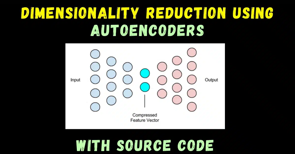
Dimensionality Reduction Using Autoencoders - Easy Explanation - With Source Code - 2024

So in today’s very interesting blog, we will see that how we can perform Dimensionality Reduction using Autoencoders in the simplest way possible using Tensorflow. So without any further due, Let’s do it…

Table of Contents

Step 1 – Importing all required libraries.

import numpy as np
import pandas as pd
import matplotlib.pyplot as plt
from tensorflow.keras.layers import Dense
from tensorflow.keras.optimizers import Adam
from tensorflow.keras.models import Sequential,Model
from sklearn.preprocessing import MinMaxScaler
import seaborn as sns

%matplotlib inline

Step 2 – Reading our input data.

data = pd.read_csv('anonymized_data.csv')
data.head()

We have 30 feature columns and 1 Label column in our dataset.
These feature columns are anonymous.

Dimensionality Reduction using Autoencoders

Step 3 – Checking info of our data.

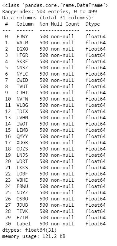
data.info()

We can see from the stats below that we don’t have any null values in our data.

Dimensionality Reduction using Autoencoders info — Information of our data

Step 4 – Scaling our data for Dimensionality Reduction using Autoencoders.

scaler = MinMaxScaler()
scaled_data = scaler.fit_transform(data.drop('Label',axis=1))
scaled_data.shape

We are using MinMaxScaler here to scale our data.
Also here we are checking the shape of our data.
While scaling we dropped the Label column as shown above.

Step 5 – Defining no. of nodes in layers.

num_inputs = 30
num_hidden = 2 
num_outputs = num_inputs # Must be true for an autoencoder!

Step 6 – Building the model for Dimensionality Reduction using Autoencoders.

model = Sequential()

model.add(Dense(num_inputs, input_shape=[num_inputs]))
model.add(Dense(num_hidden))
model.add(Dense(num_outputs))

model.compile(optimizer=Adam(0.001), metrics=['accuracy'], loss='mae')

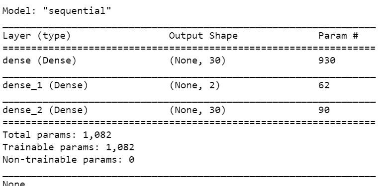
print(model.summary())

We have a very simple model for this use case.
We have 3 layers.
The first layer is having 30 nodes, 2nd is having 2 nodes and the third is also having 30 nodes.
Our input and output nodes should show the same type of data when building Autoencoders.

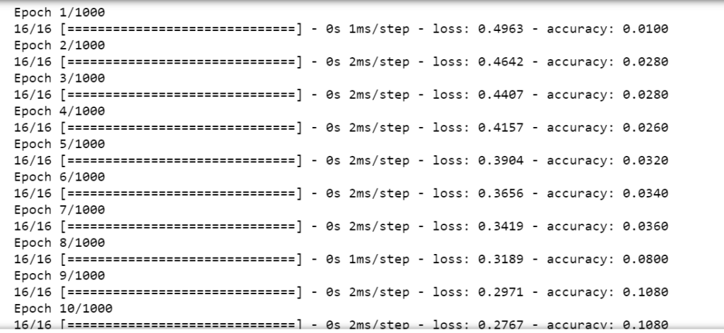
Dimensionality Reduction using Autoencoders model summary

Step 7 – Let’s train the model for Dimensionality Reduction using Autoencoders.

model.fit(x=scaled_data, y=scaled_data, epochs=1000, batch_size=32)

Step 8 – Take the output from the middle layer.

intermediate_layer_model = Model(inputs=model.input, outputs=model.get_layer(index=1).output)
intermediate_output = intermediate_layer_model.predict(scaled_data)

We can’t just directly take the output from our middle layer.
That’s why we need to create a model, with just 1 layer which will be our middle layer.
model.get_layer(index=1) is extracting the middle layer from our original model and .output is used for taking its output.
In the second line, we are simply using predict to take the results from the 2nd layer.

Step 9 – Checking the output shape of our result.

intermediate_output.shape

As we can see below that the shape of the intermediate output became 500X2 means 30 columns/features are now suppressed to only 2 columns/features.

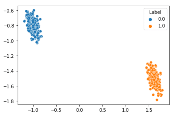
Step 10 – Plotting our results for Dimensionality Reduction using Autoencoders.

sns.scatterplot(intermediate_output[:,0],intermediate_output[:,1],hue=data['Label'])

And BOOM here is the result.
The amount of data our 30 features were showing, we are able to show that data precisely using just these 2 dimensions.
Both classes are linearly separable, which means our model did a good job of keeping the essence of the data.