How To Detect Edges Using Laplacian 2nd Order Derivative In Python Using OpenCV - Easy Project - 2024

In today’s blog of this OpenCV series, we are going to implement a Laplacian High Pass Filter or Laplacian 2nd order derivative for images which is a very useful image processing mostly used in defense domains (in missiles or tanks) to track down enemy’s tanks and trucks and destroy them.

This is going to be a very interesting blog, so without any further due, Let’s do it…

Table of Contents

Step 1 – Import the libraries required for Laplacian 2nd order derivative.

import cv2
import matplotlib.pyplot as plt

Step 2 – Read the image.

img = cv2.imread('4.tiff')
img = cv2.cvtColor(img, cv2.COLOR_BGR2RGB)

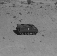
Laplacian 2nd order derivative — Read the image

After reading, we are converting the image from BGR to RGB, because we know that cv2 automatically reads the image in BGR format, whereas the images are in RGB format originally.
That’s why we need to convert it back.

Step 3 – Let’s Blur the Image to remove noise.

img = cv2.GaussianBlur(img,(13,13),0)

Here we are using Gaussian Blur to remove the Gaussian Noise from the image.
We are doing this because Laplacian is a second-order derivative operation and it is very sensitive to noise.

Step 4 – Pass the image through the Laplacian 2nd order derivative.

Syntax: cv2.Laplacian(src, ddepth[, ksize[, scale[, delta[, borderType]]]]])

Parameters:

src	Source image.
ddepth	Desired depth of the destination image.
ksize	Aperture size used to compute the second-derivative filters. See getDerivKernels for details. The size must be positive and odd.
scale	Optional scale factor for the computed Laplacian values. By default, no scaling is applied. See getDerivKernels for details.
delta	Optional delta value that is added to the results prior to storing them in dst .
borderType	Pixel extrapolation method.

edges = cv2.Laplacian(img, -1, ksize=5, scale=1, delta=0,borderType=cv2.BORDER_DEFAULT)

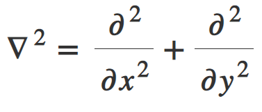
The Laplacian function calculates the Laplacian of the source image by adding up the second x and y derivatives calculated using the Sobel operator.
Unlike first-order filters that detect the edges based on local maxima or minima, Laplacian detects the edges at zero crossings i.e. where the value of the derivative changes from negative to positive and vice-versa.
Remember Sobel X and Sobel Y are first-order derivatives in the X and Y direction respectively and on the other hand, Laplacian is a sum of second-order derivatives in the X and Y directions.

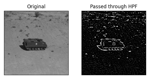
Step 5 – Let’s plot the results.

output = [img, edges]
titles = ['Original', 'Passed through HPF']

for i in range(2):
    plt.subplot(1, 2, i + 1)
    plt.imshow(output[i], cmap='gray')
    plt.title(titles[i])
    plt.xticks([])
    plt.yticks([])
plt.show()

NOTE – You can read more bout Laplace Operator here.

Let’s see the whole code for the Laplacian 2nd order derivative…

# Laplacian 2nd order derivative
import cv2
import matplotlib.pyplot as plt

img = cv2.imread('4.tiff')
img = cv2.cvtColor(img, cv2.COLOR_BGR2RGB)

blur_img = cv2.GaussianBlur(img, (13, 13), 0)

edges = cv2.Laplacian(blur_img, -1, ksize=5, scale=1, delta=0, borderType=cv2.BORDER_DEFAULT)

output = [img, edges]
titles = ['Original', 'Passed through HPF']

for i in range(2):
    plt.subplot(1, 2, i + 1)
    plt.imshow(output[i], cmap='gray')
    plt.title(titles[i])
    plt.xticks([])
    plt.yticks([])
plt.show()

Do let me know if there’s any query regarding Laplacian 2nd order derivative by contacting me by email or LinkedIn.

So this is all for this blog folks, thanks for reading it and I hope you are taking something with you after reading this and till the next time ?…

Read my previous post: HOW TO PLOT A HISTOGRAM OF A GRAYSCALE IMAGE IN 2 WAYS IN PYTHON USING OPENCV

Check out my other machine learning projects, deep learning projects, computer vision projects, NLP projects, Flask projects at machinelearningprojects.net.