How to generate negative images in Python using OpenCV – interesting project – 2024

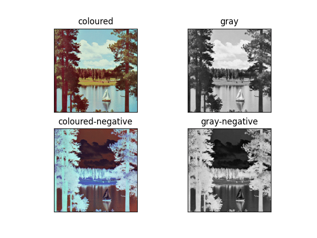
So, in today’s blog of this OpenCV series, we are going to generate a negative image. Talking about negatives, it’s a very nostalgic feeling because nowadays we are not used to seeing negatives but about 10-15 years ago, first of all, negatives were generated, and then the original images.

This is going to be a very interesting blog, so without any further due, Let’s do it…

Step 1 – Import libraries.

import cv2
import matplotlib.pyplot as plt

Step 2 – Let’s read the image.

imgpath = 'test.tiff'
img = cv2.imread(imgpath)

Step 3 – Convert the image to RGB

img = cv2.cvtColor(img, cv2.COLOR_BGR2RGB)

• Here we are just converting the image from BGR to RGB because cv2 reads the image in BGR format by default.
• That’s why we need to convert it back to RGB format.

Step 4 – Let’s read the image in grayscale also.

gray = cv2.imread(imgpath, 0)

We are also reading the image in grayscale mode to generate its negative.

Step 5 – Lets generate the negative image.

Algorithm of finding the negative:

• Get the red green blue values of each pixel.
• Subtract each color value from 255 and save them as new color values.
• Create a new pixel value from the modified colors.
• set the new value to the pixel.

colored_negative = abs(255-img)
gray_negative = abs(255-gray)

• For colored images, we will subtract 255 from all the values of all 3 channels (RGB) and take its absolute value (positive value).
• For a grayscale image, we have just 1 channel and there also we will subtract 255 from those pixel values (pixel value ranges from 0-255 in grayscale images) and take absolute values.
• We can consider negative images as the exact opposite of the original images, if we add both, the original image and the negative image, we will get a pure white image.

Step 6 – Let’s plot the results.

imgs = [img, gray, colored_negative, gray_negative]
title = ['coloured', 'gray', 'coloured-negative', 'gray-negative']


plt.subplot(2, 2, 1)
plt.title(title[0])
plt.imshow(imgs[0])
plt.xticks([])
plt.yticks([])

plt.subplot(2, 2, 2)
plt.title(title[1])
plt.imshow(imgs[1], cmap='gray')
plt.xticks([])
plt.yticks([])

plt.subplot(2, 2, 3)
plt.title(title[2])
plt.imshow(imgs[2])
plt.xticks([])
plt.yticks([])

plt.subplot(2, 2, 4)
plt.title(title[3])
plt.imshow(imgs[3], cmap='gray')
plt.xticks([])
plt.yticks([])

plt.show()

Let’s see the whole code…

import cv2
import matplotlib.pyplot as plt

imgpath = '4.2.06.tiff'
img = cv2.imread(imgpath)

img = cv2.cvtColor(img1, cv2.COLOR_BGR2RGB)

gray = cv2.imread(imgpath, 0)


colored_negative  = abs(255-img1)
gray_negative  = abs(255-gray)

imgs = [img, gray, colored_negative, gray_negative]
title = ['coloured', 'gray', 'coloured-negative', 'gray-negative']

plt.subplot(2, 2, 1)
plt.title(title[0])
plt.imshow(imgs[0])
plt.xticks([])
plt.yticks([])

plt.subplot(2, 2, 2)
plt.title(title[1])
plt.imshow(imgs[1], cmap='gray')
plt.xticks([])
plt.yticks([])

plt.subplot(2, 2, 3)
plt.title(title[2])
plt.imshow(imgs[2])
plt.xticks([])
plt.yticks([])

plt.subplot(2, 2, 4)
plt.title(title[3])
plt.imshow(imgs[3], cmap='gray')
plt.xticks([])
plt.yticks([])

plt.show()

Note – Read more about negative images.

Do let me know if there’s any query regarding this topic by contacting me by email or LinkedIn.

So this is all for this blog folks, thanks for reading it and I hope you are taking something with you after reading this and till the next time…

Read my previous post: HOW TO DETECT EDGES USING LAPLACIAN 2ND ORDER DERIVATIVE IN PYTHON USING OPENCV

Check out my other machine learning projects, deep learning projects, computer vision projects, NLP projects, Flask projects at machinelearningprojects.net.