So guys in today’s blog we will implement the Milk Production prediction for the next year with the previous 13-year milk production data. We will use LSTM for this project because of the fact that the data is Sequential. So without any further due, Let’s do it…
Step 1 – Importing required libraries.
import numpy as np
import pandas as pd
import matplotlib.pyplot as plt
from sklearn.preprocessing import MinMaxScaler
from tensorflow.keras.models import Sequential
from tensorflow.keras.layers import LSTM,Activation,Dense,Dropout
%matplotlib inline
Step 2 – Read the input data.
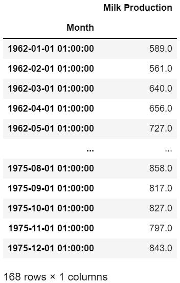
df = pd.read_csv('monthly-milk-production.csv',index_col='Month')
df.index = pd.to_datetime(df.index)
df
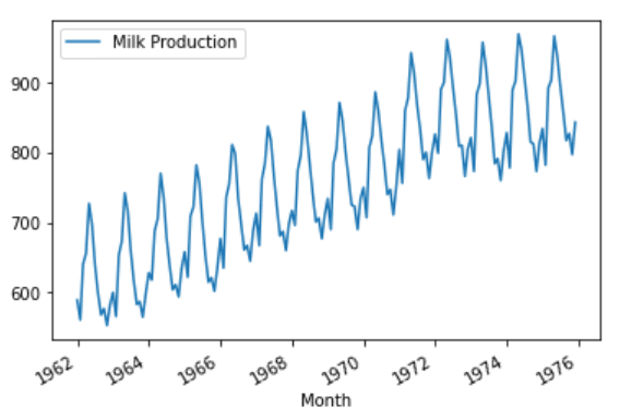
Step 3 – Plotting data.
df.plot()
Step 4 – Scaling Data.
scaler = MinMaxScaler()
array = []
train_data = []
train_labels = []
for i in range(len(df)):
array.append(df.iloc[i]['Milk Production'])
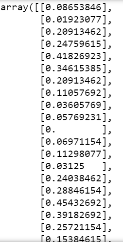
array = np.array(array).reshape(-1,1)
array = scaler.fit_transform(array)
array
- Using MinMaxScaler here to bring our data in the 0-1 range.
- Then just reshaping it to make just one column and n no. of rows where n represents the no. of elements in the array.
Step 5 – Creating training data.
k = 0
for i in range(len(array)):
    try:
        train_data.append(array[12*k:12*(k+1)])
        train_labels.append(array[12*(k+1)])
        k+=1
    except:
        break

train_data = np.squeeze(train_data)
train_labels = np.array(train_labels)

train_data.shape
- Here we are just creating training data.
- train data will have the first array as the first 12 points of the array and its corresponding train label will be the 13th entry in the array.
- In this way, we will have 14 arrays of 12 points each.
- But the training label will have only 13 points that’s why we will also take only 13 arrays in train data.

Step 6 – Getting train data in shape.
train_data = train_data[:len(train_labels)]
train_data = np.expand_dims(train_data,1)
train_data.shape
- Taking the first 13 arrays in train data.
- Then expanding dimensions in 1st dimension. We are doing this step because Keras wants the data in this format.
Step 7 – Checking train data and train labels.
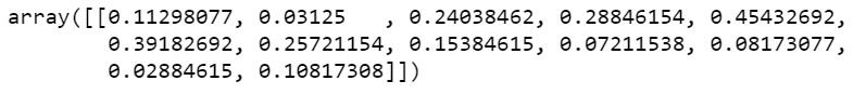
train_data[1]
- This is the first array in train_data. It shows the milk production of 12 months.
- And its corresponding train label will be the milk production of the 13th month, which means the first month of next year.
- We will train our data on 12 months’ data and ask our model to predict the production of the 13th month (1st month of next year).
train_labels[1]
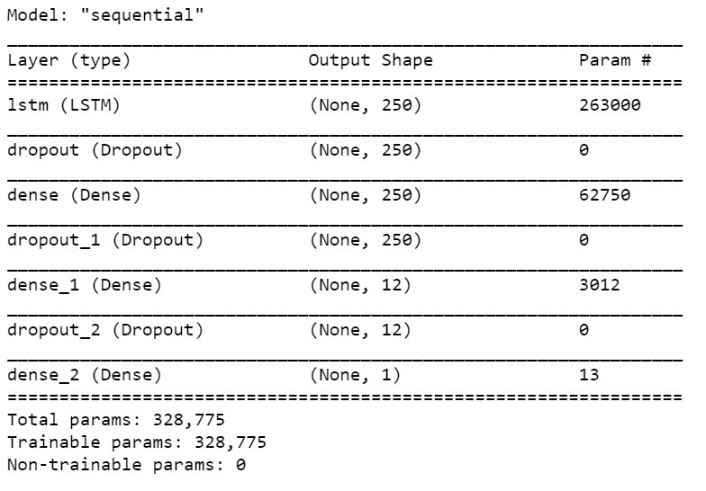
Step 8 – Creating a model.
model = Sequential()

model.add(LSTM(250,input_shape=(1,12)))
model.add(Dropout(0.5))


model.add(Dense(250,activation='relu'))
model.add(Dropout(0.5))

model.add(Dense(12,activation='relu'))
model.add(Dropout(0.5))

model.add(Dense(1,activation='relu'))

model.compile(loss='mean_squared_error',optimizer='adam')

model.summary()
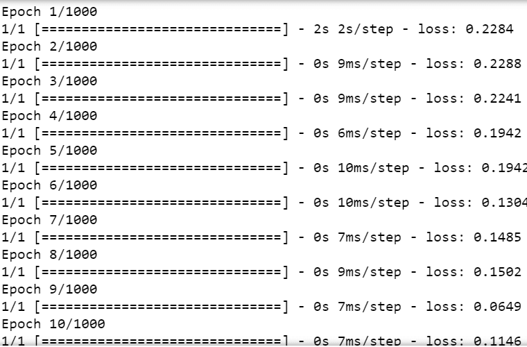
Step 9 – Training model.
E = 1000

H = model.fit(train_data,train_labels,epochs=E)
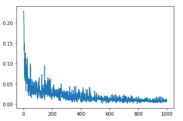
Step 10 – Plotting loss curve for Milk Production prediction model.
epochs = range(0,E)
loss = H.history['loss']
plt.plot(epochs,loss)
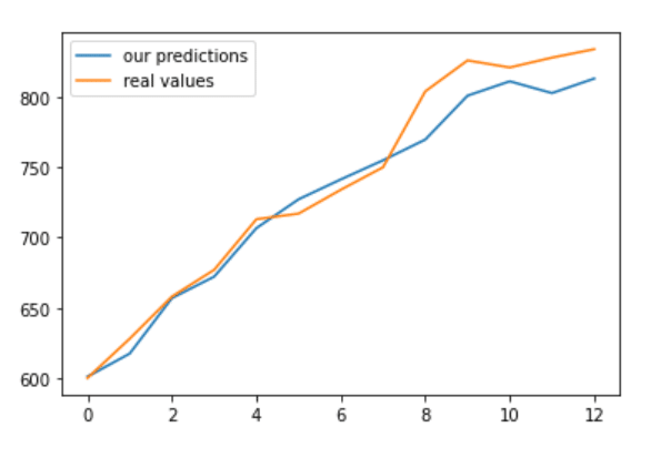
Step 11 – Checking if our Milk Production prediction model is overfitting or not.
preds = scaler.inverse_transform(model.predict(train_data))
plt.plot(range(0,13),preds,label='our predictions')
plt.plot(range(0,13),scaler.inverse_transform(train_labels),label='real values')
plt.legend()
Step 12 – Create a seed for next year’s Milk Production prediction.
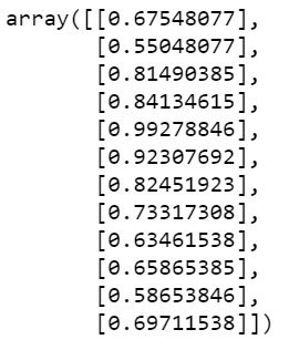
seed = array[-12:]
seed
- Here we are creating a seed which means the 12 last data points in the array. Suppose this is the milk production of 12 months of 1975.
- Now we will ask our model to predict the production for Jan 1976.
- When it will predict then we will update our seed.
- And now our seed will be Feb 1975 – Jan 1976 and we will ask our model to predict for Feb 2022.
- And in this way, we will predict for full 1976.
- This is all done below.
seed.shape

Step 13 – Next year’s Milk Production prediction.
for _ in range(12):
curr_12_months = seed[-12:]
curr_12_months = np.squeeze(curr_12_months)
curr_12_months = np.expand_dims(curr_12_months,0)
curr_12_months = np.expand_dims(curr_12_months,0)
pred = model.predict(curr_12_months)
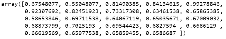
seed = np.append(seed,pred)
seed
- This step is explained above.
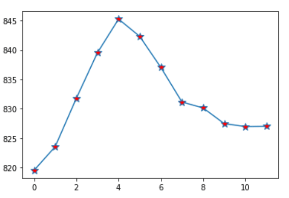
Step 14 – Plotting next year’s Milk Production prediction.
next_year_prediction = scaler.inverse_transform(seed[-12:].reshape(-1,1))
plt.plot(range(0,12),next_year_prediction,marker='*',markerfacecolor='red',markersize=10)
- This is the production of 1976.
Download Source Code…
Do let me know if there’s any query regarding the Milk Production prediction by contacting me on email or LinkedIn. You can also comment down below for any queries.
So this is all for this blog folks, thanks for reading it and I hope you are taking something with you after reading this and till the next time ?…
Read my previous post: AI LEARNS TO PLAY FLAPPY BIRD GAME
Check out my other machine learning projects, deep learning projects, computer vision projects, NLP projects, Flask projects at machinelearningprojects.net.