In today’s blog, we are going to find the most dominant colors in an image, this is going to be a very interesting blog because the project which we are going to build today is very simple and powerful. So without any further due, Let’s do it…
Checkout the video here – https://youtu.be/AAmye1qwwwQ
Code for the most dominant colors in an image…
import cv2
import numpy as np
import matplotlib.pyplot as plt
from sklearn.cluster import KMeans
import imutils
clusters = 5 # try changing it
img = cv2.imread('5.png')
org_img = img.copy()
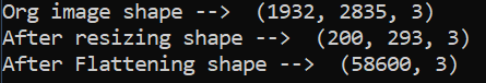
print('Org image shape --> ',img.shape)
img = imutils.resize(img,height=200)
print('After resizing shape --> ',img.shape)
flat_img = np.reshape(img,(-1,3))
print('After Flattening shape --> ',flat_img.shape)
kmeans = KMeans(n_clusters=clusters,random_state=0)
kmeans.fit(flat_img)
dominant_colors = np.array(kmeans.cluster_centers_,dtype='uint')
percentages = (np.unique(kmeans.labels_,return_counts=True)[1])/flat_img.shape[0]
p_and_c = zip(percentages,dominant_colors)
p_and_c = sorted(p_and_c,reverse=True)
block = np.ones((50,50,3),dtype='uint')
plt.figure(figsize=(12,8))
for i in range(clusters):
plt.subplot(1,clusters,i+1)
block[:] = p_and_c[i][1][::-1] # we have done this to convert bgr(opencv) to rgb(matplotlib)
plt.imshow(block)
plt.xticks([])
plt.yticks([])
plt.xlabel(str(round(p_and_c[i][0]*100,2))+'%')
bar = np.ones((50,500,3),dtype='uint')
plt.figure(figsize=(12,8))
plt.title('Proportions of colors in the image')
start = 0
i = 1
for p,c in p_and_c:
end = start+int(p*bar.shape[1])
if i==clusters:
bar[:,start:] = c[::-1]
else:
bar[:,start:end] = c[::-1]
start = end
i+=1
plt.imshow(bar)
plt.xticks([])
plt.yticks([])
rows = 1000
cols = int((org_img.shape[0]/org_img.shape[1])*rows)
img = cv2.resize(org_img,dsize=(rows,cols),interpolation=cv2.INTER_LINEAR)
copy = img.copy()
cv2.rectangle(copy,(rows//2-250,cols//2-90),(rows//2+250,cols//2+110),(255,255,255),-1)
final = cv2.addWeighted(img,0.1,copy,0.9,0)
cv2.putText(final,'Most Dominant Colors in the Image',(rows//2-230,cols//2-40),cv2.FONT_HERSHEY_DUPLEX,0.8,(0,0,0),1,cv2.LINE_AA)
start = rows//2-220
for i in range(5):
end = start+70
final[cols//2:cols//2+70,start:end] = p_and_c[i][1]
cv2.putText(final,str(i+1),(start+25,cols//2+45),cv2.FONT_HERSHEY_DUPLEX,1,(255,255,255),1,cv2.LINE_AA)
start = end+20
plt.show()
cv2.imshow('img',final)
cv2.waitKey(0)
cv2.destroyAllWindows()
cv2.imwrite('output.png',final)
- Line 1-5 – Importing packages required to find most dominant colors in an image.
- Line 7 – Defining the no. of clusters for the KMeans algorithm.
- Line 9 – Reading our input image.
- Line 10 – Keeping a copy of it for future use.
- Line 11 – Printing its shape.
- Line 13 – Resizing our image to get results fast.
- Line 14 – Printing resized image shape.
- Line 16 – Flattening the image. In this step, we are just keeping all the columns of the image after each other to make just one column out of it. After this step, we will be left with just 1 column and rows equal to the no. of pixels in the image.
- Line 17 – Let’s check the shape of the flattened image now.
- Line 19 – Making a KMeans Clustering object with n_clusters set to 5 as declared in Line 7.
- Line 20 – Fit our image in Kmeans Clustering Algorithm. In this step, the flattened image is working as an array containing all the pixel colors of the image. These pixel colors will now be clustered into 5 groups. These groups will have some centroids which we can think of as the major color of the cluster (In Layman’s terms we can think of it as the boss of the cluster).
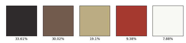
- Line 22 – We are extracting these cluster centers. Now we know that these 5 colors are the dominant colors of the image but still, we don’t know the extent of each color’s dominance.
- Line 24 – We are calculating the dominance of each dominant color. np.unique(kmeans.labels_,return_counts=True), this statement will return an array with 2 parts, first part will be the predictions like [2,1,0,1,4,3,2,3,4…], means to which cluster that pixel belongs and the second part will contain the counts like [100,110,310,80,400] where 100 depicts the no. of pixels belonging to class 0 or cluster 0(our indexing starts from 0), and so on, and then we are simply dividing that array by the total no. of pixels, 1000 in the above case, so the percentage array becomes [0.1,0.11,0.31,0.08,0.4]
- Line 25 – We are zipping percentages and colors together like, [(0.1,(120,0,150)), (0.11,(230,225,34)), …]. It will consist of 5 tuples. First tuple is (0.1,(120,0,150)) where first part of the tuple (0.1) is the percentage and (120,0,150) is the color.
- Line 26 – Sort this zip object in descending order. Now the first element in this sorted object will be the percentage of the most dominant colors in the image and the color itself.
- Line 28-36 – We are plotting blocks of dominant colors.
- Line 38-54 – We are plotting the following bar.

- Line 56-72 – We are creating the final result.
- Line 79- We are saving the output image.
Final Results of most dominant colors in an image…

NOTE 1 – You can skip the bar and blocks part as they are just some visualizations for better understanding.
NOTE 2 – You can always try and play with cluster no. in Line 7 but the no. of blocks on the final image can only go max up to 5.
Download the Source Code…
Do let me know if there’s any query regarding the most dominant colors in an image by contacting me on email or LinkedIn.
So this is all for this blog folks, thanks for reading it and I hope you are taking something with you after reading this and till the next time ?…
Read my previous post: HOW TO PERFORM FACE RECOGNITION USING KNN
Check out my other machine learning projects, deep learning projects, computer vision projects, NLP projects, Flask projects at machinelearningprojects.net.
The project documentation for the Find most dominant color in an image using k-means algorithm project