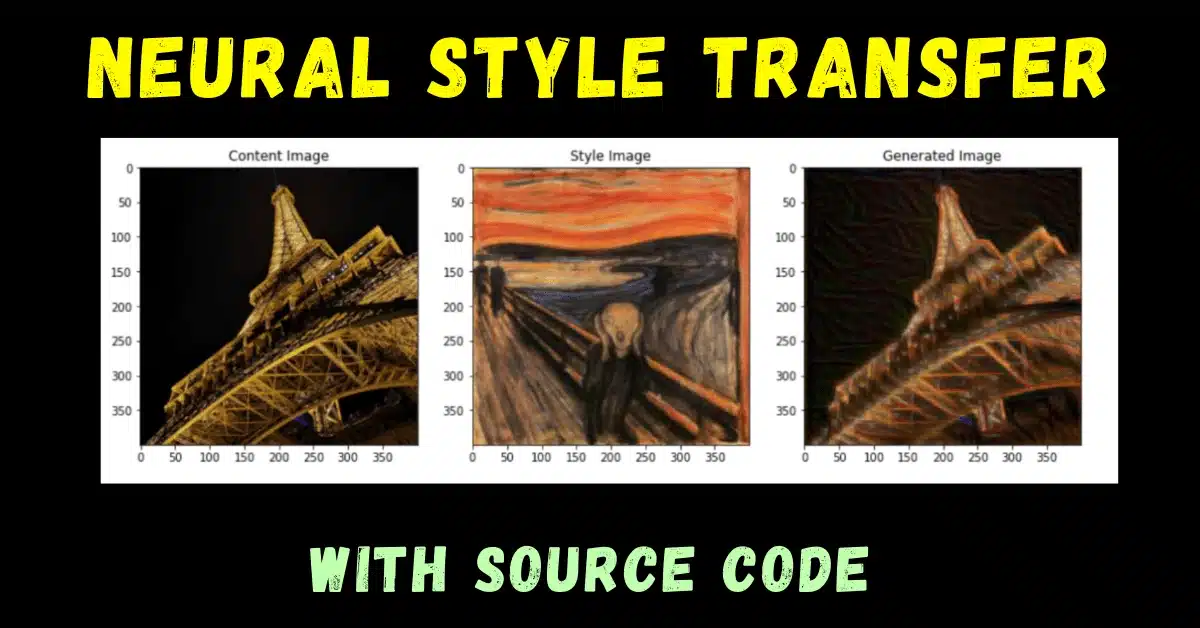
Who said that only humans can create beautiful artwork? In today’s blog, we will see how a neural network application called Neural Style Transfer can create beautiful artworks which even humans can’t think of. So without any due, Let’s do it…
Step 1 – Importing Libraries required for Neural Style Transfer.
import time
import imageio
import numpy as np
import tensorflow as tf
from matplotlib import pyplot as plt
from scipy.optimize import fmin_l_bfgs_b
from tensorflow.keras import backend as K
from tensorflow.keras.applications import vgg16
from tensorflow.keras.preprocessing.image import load_img, img_to_array

tf.compat.v1.disable_eager_execution()

%matplotlib inline
Step 2 – Read the content and style images.
# This is the path to the image you want to transform.
target_image_path = './images/eiffel.jpg'

# This is the path to the style image.
style_reference_image_path = './images/thescream.jpg'

result_prefix = style_reference_image_path.split("images/")[1][:-4] + '_onto_' + target_image_path.split("images/")[1][:-4]

# Dimensions of the generated picture.
width, height = load_img(target_image_path).size
img_height = 400
img_width = int(width * img_height / height)

def preprocess_image(image_path):
    img = load_img(image_path, target_size=(img_height, img_width))
    img = img_to_array(img)
    img = np.expand_dims(img, axis=0)
    img = vgg16.preprocess_input(img)
    return img

def deprocess_image(x):
    # Remove zero-center by mean pixel and adding standardizing values to B,G,R channels respectively
    x[:, :, 0] += 103.939
    x[:, :, 1] += 116.779
    x[:, :, 2] += 123.68
    # 'BGR'->'RGB'
    x = x[:, :, ::-1]
    x = np.clip(x, 0, 255).astype('uint8') # limits the value of x between 0 and 255
    return x
Step 3 – Defining some utility functions for Neural Style Transfer.
def content_loss(target, final):
    return K.sum(K.square(target-final))

def gram_matrix(x):
    features = K.batch_flatten(K.permute_dimensions(x, (2, 0, 1)))
    gram = K.dot(features, K.transpose(features))
    return gram

def style_loss(style, final_img):
    S = gram_matrix(style)
    F = gram_matrix(final_img)
    channels = 3
    size = img_height * img_width
    return K.sum(K.square(S - F)) / (4. * (channels ** 2) * (size ** 2))

def total_variation_loss(x):
    a = K.square(x[:, :img_height - 1, :img_width - 1, :] - x[:, 1:, :img_width - 1, :])
    b = K.square(x[:, :img_height - 1, :img_width - 1, :] - x[:, :img_height - 1, 1:, :])
    return K.sum(K.pow(a + b, 1.25))
Step 4 – Loading the VGG model for Neural Style Transfer.
# load reference image and style image
target_image = K.constant(preprocess_image(target_image_path))
style_reference_image = K.constant(preprocess_image(style_reference_image_path))

# This placeholder will contain our final generated image
final_image = K.placeholder((1, img_height, img_width, 3))

# We combine the 3 images into a single batch
input_tensor = K.concatenate([target_image,
                              style_reference_image,
                              final_image], axis=0)

# We build the VGG16 network with our batch of 3 images as input.
# The model will be loaded with pre-trained ImageNet weights.
model = vgg16.VGG16(input_tensor=input_tensor,
                    weights='imagenet',
                    include_top=False)

print('Model loaded.')
Step 5 – Computing losses of Neural Style Transfer model.
# creatin a dictionary containing layer_name:layer_output
outputs_dict = dict([(layer.name, layer.output) for layer in model.layers])

# Name of layer used for content loss
content_layer = 'block5_conv2'

# Name of layers used for style loss
style_layers = ['block1_conv1',
                'block2_conv1',
                'block3_conv1',
                'block4_conv1',
                'block5_conv1']

# Weights in the weighted average of the loss components
total_variation_weight = 1e-4 #(randomly taken)
style_weight = 1.             #(randomly taken)
content_weight = 0.025        #(randomly taken)

# Define the loss by adding all components to a `loss` variable
loss = K.variable(0.)
layer_features = outputs_dict[content_layer]
target_image_features = layer_features[0, :, :, :] #as we concatenated them above and here 1 will be style fetures
combination_features = layer_features[2, :, :, :]
loss = loss + content_weight * content_loss(target_image_features,combination_features)# adding content loss

for layer_name in style_layers:

    layer_features = outputs_dict[layer_name]

    style_reference_features = layer_features[1, :, :, :]
    combination_features = layer_features[2, :, :, :]

    sl = style_loss(style_reference_features, combination_features)
    loss += sl * (style_weight / len(style_layers))      #adding style loss

loss += total_variation_weight * total_variation_loss(final_image)

# Get the gradient of the loss wrt the final image means how is loss changing wrt final image
grads = K.gradients(loss, final_image)[0]

# Function to fetch the values of the current loss and the current gradients
fetch_loss_and_grads = K.function([final_image], [loss, grads])
Step 6 – Defining Evaluator class.
class Evaluator(object):

    def __init__(self):
        self.loss_value = None
        self.grads_values = None

    def loss(self, x):
        assert self.loss_value is None
        x = x.reshape((1, img_height, img_width, 3))
        outs = fetch_loss_and_grads([x])
        loss_value = outs[0]
        grad_values = outs[1].flatten().astype('float64')
        self.loss_value = loss_value
        self.grad_values = grad_values
        return self.loss_value

    def grads(self, x):
        assert self.loss_value is not None
        grad_values = np.copy(self.grad_values)
        self.loss_value = None
        self.grad_values = None
        return grad_values

evaluator = Evaluator()
Step 7 – Training our Neural Style Transfer model.
# After 10 iterations little change occurs
iterations = 10
# Run scipy-based optimization (L-BFGS) over the pixels of the generated image so as to minimize the neural style loss.
# This is our initial state: the target image.
# Note that `scipy.optimize.fmin_l_bfgs_b` can only process flat vectors.
x = preprocess_image(target_image_path)
x = x.flatten()
# fmin_l_bfgs_b(func,x) minimizes a function func using the L-BFGS-B algorithm where
# x is the initial guess
# fprime is gradient of the function
# maxfun is Maximum number of function evaluations.
# returns x which is Estimated position of the minimum.
# minval -> Value of func at the minimum.
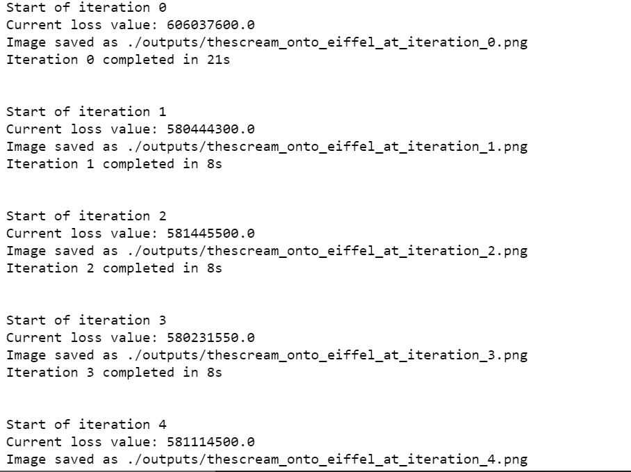
for i in range(iterations):
print('Start of iteration', i)
start_time = time.time()
estiated_min, func_val_at_min, info = fmin_l_bfgs_b(evaluator.loss, x,fprime=evaluator.grads, maxfun=20)
print('Current loss value:', func_val_at_min)
# Save current generated image
img = estiated_min.copy().reshape((img_height, img_width, 3))
img = deprocess_image(img)
fname = "./outputs/" + result_prefix + '_at_iteration_%d.png' % i
imageio.imwrite(fname, img)
end_time = time.time()
print('Image saved as', fname)
print('Iteration %d completed in %ds' % (i, end_time - start_time))
print('\n')
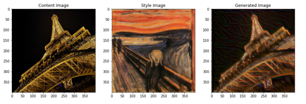
Step 8 – Visualizing the Neural Style Transfer results.
plt.figure(figsize=(15,8))

# Content image
plt.subplot(131)
plt.title('Content Image')
plt.imshow(load_img(target_image_path, target_size=(img_height, img_width)))

# Style image
plt.subplot(132)
plt.title('Style Image')
plt.imshow(load_img(style_reference_image_path, target_size=(img_height, img_width)))

# Generate image
plt.subplot(133)
plt.title('Generated Image')
plt.imshow(img)
Download Source Code for Neural Style Transfer…
Do let me know if there’s any query regarding the Neural Style Transfer by contacting me by email or LinkedIn. You can also comment down below for any queries.
So this is all for this blog folks, thanks for reading it and I hope you are taking something with you after reading this and till the next time ?…
Read my previous post: SUDOKU SOLVER – WITH SOURCE CODE
Check out my other machine learning projects, deep learning projects, computer vision projects, NLP projects, Flask projects at machinelearningprojects.net.